Population Stability Index gets more attention in model monitoring than it deserves, and vintage analysis gets less. PSI tells you that your applicant population has shifted. It doesn't tell you whether your model is still ranking risk correctly within the shifted population. It doesn't tell you whether the rate of charge-offs in a specific origination cohort has changed relative to what the model predicted when those loans were booked. And it certainly doesn't give you the 6-to-12-month early warning signal that allows a credit team to adjust policy before the charge-off wave arrives — rather than after it's already visible in the portfolio.
Vintage analysis at the decision layer is what fills that gap. It's not a new methodology — vintage cohort tracking has been standard practice in consumer credit management since the 1990s. What's changed is where the analysis needs to happen and what data it needs to draw on to be actionable. When decisioning is done through an orchestration layer that logs both model scores and decision reasons at origination, you have the inputs to do vintage analysis at a level of granularity that most lenders' current monitoring workflows don't approach.
Vintage Curves and Why They're Not Just for Portfolio Reporting
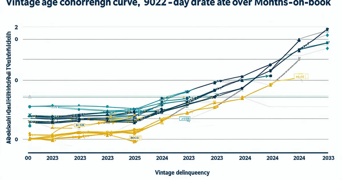
A vintage curve plots the cumulative charge-off rate of an origination cohort — all loans originated in a given month or quarter — against months on book. A typical near-prime consumer installment portfolio sees charge-offs begin ramping at 3 to 6 months on book, peak in the 12-to-18-month range, and level off as the cohort seasons past 24 months. The shape of the curve, and its level at any given month on book, tells you two things: how the cohort is performing, and how it's performing relative to the model's predictions at the time of origination.
The second comparison is the one most lenders underinvest in. If your model predicted a 4.8% charge-off rate for Q1 2024 originations at 18 months on book, and the Q1 2024 vintage is running at 6.1% by month 12 on an early-curve basis, that's not just a portfolio management problem — it's a model calibration problem. The model's probability estimates for that cohort were wrong, and if you're still using the same model for current originations, you're accepting risk premiums calibrated against a prediction that proved inaccurate.
Connecting vintage performance back to the decision layer requires that the origination record for each loan include the decision factors at origination: the model score, the score band, and the primary decision reason codes. Without that connection, you can observe that a cohort is underperforming, but you can't diagnose which segment of the cohort is driving the underperformance — whether it's concentrated in a specific score band, driven by a specific policy pathway, or spread uniformly across the cohort.
PSI as the Trip Wire — Not the Diagnosis
PSI thresholds — 0.10 as a monitoring alert, 0.25 as a review trigger — are useful early indicators of population shift, but they're not a substitute for cohort-level outcome analysis. A PSI of 0.12 on your primary score distribution tells you that your current applicant mix is meaningfully different from the model's development sample. It doesn't tell you whether the model's rank-ordering is still accurate within the new distribution.
The scenario where PSI fails as a sole monitoring metric: an online installment lender running approximately 120,000 originations per year whose applicant mix shifted toward higher average FICO scores during late 2022 as other lenders tightened their credit standards. PSI on the score distribution would have flagged that shift — the distribution moved up, PSI was 0.14, above the alert threshold. But the lender's model had been trained on a mixed near-prime and subprime population. In the higher-FICO band, the model's calibration was less precise — it had seen fewer training examples in that range, and its probability estimates for those applicants were less reliable. The PSI alert said "your population shifted." The vintage analysis, which the lender did 18 months later when early charge-off rates in the Q3 2022 cohort came in above the model's predictions, said "your model's calibration in the 680-to-720 FICO band was miscalibrated for the population you were actually originating."
Had the lender been running vintage analysis against decision-layer outputs from origination, the miscalibration signal would have been visible in the Q4 2022 cohort's 3-to-6-month early delinquency rates — well before the full charge-off outcome seasoned. The early warning time advantage is typically 9 to 12 months on a consumer installment portfolio. That's the window to adjust policy before the charge-off wave.
Cohort Definition: Where Vintage Analysis Gets Precise
Standard vintage analysis cohorts are defined by origination period — all loans funded in a given month or quarter. That's a useful starting point. Decision-layer vintage analysis adds a second dimension: cohort by model pathway. Not just "loans funded in Q1 2024" but "loans funded in Q1 2024 through the primary score pathway, score band 640-679" or "loans funded in Q1 2024 through the augmentation overlay, with FICO score 660-699 and augmentation score above the 70th percentile."
This granularity is only achievable if the decision layer logged the pathway at origination. When it did, the vintage analysis can answer questions that portfolio-level reporting can't: Is the deterioration in the Q1 2024 cohort concentrated in loans that came through the augmentation overlay? Are the loans that were approved on the basis of the manual review queue underperforming versus those that were auto-approved by the rules engine? Is there a specific bureau tradeline pattern — rapid account opening, recent derogatory mark, high revolving utilization — that predicts early delinquency disproportionately in recent vintages even after controlling for the model score?
A cohort defined by decision pathway, not just origination period, is what turns vintage analysis from a lagging report into an actionable diagnostic. The credit policy team can see which pathway is generating the underperformance, and they can adjust that pathway specifically — tightening a threshold, adding a verification requirement, adjusting a pricing tier — without modifying the entire policy or requiring a full model retrain.
Seasoning Effects and the Problem of Premature Conclusions
A critical methodological caution on vintage analysis: seasoning effects are real, and comparing vintages at different points on book requires accounting for where each cohort is in its maturity curve. A Q1 2025 vintage at 3 months on book will almost always show lower cumulative charge-offs than a Q1 2024 vintage at 15 months on book. That comparison tells you nothing useful about relative credit quality — it tells you only that newer loans have had less time to charge off.
We are not saying that early-period delinquency rates are unreliable indicators of vintage quality. We are saying that the comparison has to be cohort-to-cohort at matched months on book. Comparing Q1 2025 at 3 months to Q1 2024 at 3 months is useful. Comparing Q1 2025 at 3 months to Q1 2023 at 18 months is misleading and will produce incorrect conclusions about whether recent origination quality has improved or deteriorated.
Charge-off recovery rates add a second layer of complexity. A cohort with a 7% gross charge-off rate at 18 months on book but a 35% recovery rate has a 4.55% net charge-off rate. Another cohort with a 6% gross charge-off rate but a 15% recovery rate has a 5.1% net charge-off rate. The gross comparison would rank the first cohort as worse. The net comparison shows the opposite. For most operational credit policy purposes, net charge-off is the relevant metric — but recovery rates vary materially across product type, secured versus unsecured, and economic cycle, which means both the numerator and denominator of the performance calculation need to be tracked at the cohort level.
Integrating KS Monitoring with Vintage Tracking
A complete model monitoring program at the decision layer combines PSI for population shift detection, KS monitoring for rank-order performance, and vintage cohort tracking for outcome calibration. These three metrics answer different questions and are not substitutable for each other.
PSI answers: is the applicant population we're scoring today similar to the population the model was trained on? KS answers: is the model still ranking risk correctly within the current applicant population? Vintage answers: are the probability estimates the model produced at origination consistent with the actual outcomes we're observing as those loans mature?
In practice, the KS statistic on a model run against early delinquency outcomes at 3 to 6 months on book gives you a leading indicator of vintage performance that's meaningfully faster than waiting for the full charge-off curve to season. A model that's maintaining KS above a 0.35 threshold on early delinquency outcomes in recent cohorts is behaving consistently with its development-period performance. A model whose KS on early delinquency outcomes in Q4 2024 cohorts has fallen to 0.24 — even if the PSI looks fine — is telling you something important: its rank-ordering is degrading, and the vintage analysis is likely to confirm that the calibration is off before the charge-off signal is visible at the full-maturity level.
What Decision-Layer Logging Needs to Support This Analysis
The vintage analysis program described here requires three things from the decision layer at origination time. First, the model score and score band at origination, stored with the loan record, not just in the model log. Second, the decision pathway — which rules fired, which scoring layer was invoked, which threshold condition produced the outcome. Third, the top adverse action reason codes for declined applications, and for approved applications, the top contributing factors, stored in a format that supports cohort-level aggregation.
Without this logging, vintage analysis is limited to portfolio-level outcome tracking — useful, but not actionable at the policy-adjustment level. With it, the credit team has a continuous early warning system that connects current origination decisions to future performance outcomes, closes the feedback loop that model monitoring requires, and provides the documentation the model risk committee needs to assess whether the current model is performing within tolerance or is a candidate for retrain or replacement.
The lenders who will catch the next charge-off wave early are those who've built the cohort tracking into the decision layer itself, not those who are running the analysis retrospectively in a BI tool six months after the vintage has already seasoned past the point where policy adjustment would have changed the outcome.